LC Circuit

The LC circuit is the most fundamental example. It behaves like a quantum harmonic oscillator in the quantum regime. We can test this fundamental property here.

import circuitq as cq
import numpy as np
import networkx as nx
import matplotlib.pyplot as plt

Circuit graph

The circuit consists of a linear inductance with a shunted capacity.

graph = nx.MultiGraph()
graph.add_edge(0,1, element = 'C')
graph.add_edge(0,1, element = 'L');

Symbolic Hamiltonian

The symbolic Hamiltonian contains a harmonic potential.

circuit = cq.CircuitQ(graph)
circuit.h

$\displaystyle \frac{\Phi_{1}^{2}}{2 L_{010}} + \frac{0.5 q_{1}^{2}}{C_{01}}$

$\displaystyle \frac{\Phi_{1}^{2}}{2 L_{010}} + \frac{0.5 q_{1}^{2}}{C_{01}}$

Diagonalization

h_num = circuit.get_numerical_hamiltonian(200)
eigv, eigs = circuit.get_eigensystem()

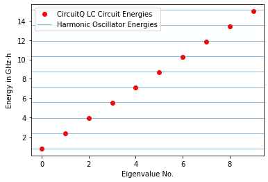
As the LC circuit represents the circuit analog of a quantum harmonic oscillator, it’s eigenenergies should be spaced by \(\hbar \omega\) with the angular frequency \(\omega = \frac{1}{\sqrt{LC}}\). We indicate these equidistant energies with horizontal lines below and plot the eigenvalues on top of them.

n_energies = 10
h = 6.62607015e-34
y_scaling = 1/(h *1e9)
plt.plot(np.arange(n_energies), eigv[:n_energies]*y_scaling,
         'ro', label='CircuitQ LC Circuit Energies')
omega = 1/np.sqrt(circuit.c_v["L"]*circuit.c_v["C"])
plt.axhline(eigv[0]*y_scaling, lw=0.5, label='Harmonic Oscillator Energies')
for n in range(1,n_energies):
    plt.axhline((eigv[0]+n*circuit.hbar*omega)*y_scaling, lw=0.5)
plt.xlabel("Eigenvalue No.")
plt.ylabel(r"Energy in GHz$\cdot$h")
plt.legend()
plt.show()

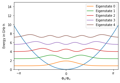
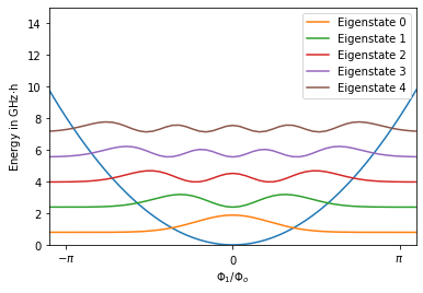
The eigenstates should have the shape of Hermite functions. Let’s plot the square of their absolute value.

plt.plot(circuit.flux_list, np.array(circuit.potential)*y_scaling, lw=1.5)
for n in range(5):
    plt.plot(circuit.flux_list,
            (eigv[n]+(abs(eigs[:,n])**2)*1e-23)*y_scaling,
            label="Eigenstate " + str(n))
plt.xticks(np.linspace(-1*np.pi, 1*np.pi, 3)*circuit.phi_0 ,
           [r'$-\pi$',r'$0$',r'$\pi$'])
plt.xlabel(r"$\Phi_1 / \Phi_o$")
plt.ylabel(r"Energy in GHz$\cdot$h")
plt.xlim(-1.1*np.pi*circuit.phi_0, 1.1*np.pi*circuit.phi_0)
plt.ylim(0,15)
plt.legend()
plt.show()